What remains useful in a neural network after it loses the task that originally trained it?

Filed under: AlexNet transfer learning Caffe scikit-learn stroke diffusion MRI ensemble learning medical imaging

Off With His Head: Transfer Learning with AlexNet

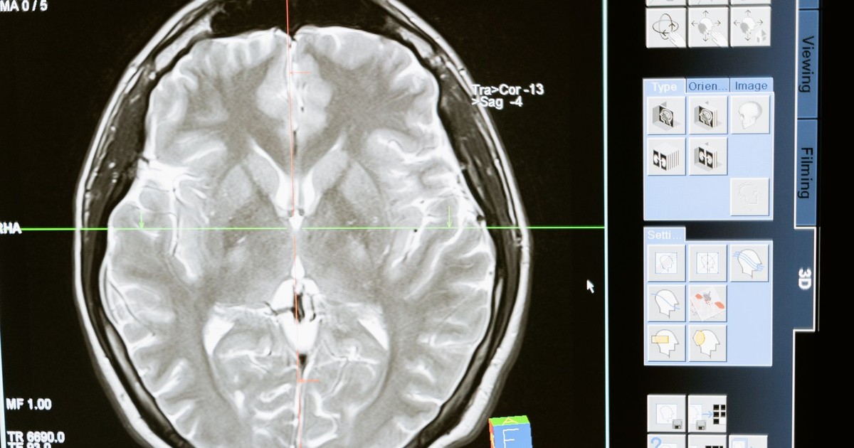
Most days, there is no neural network. There are scans, spreadsheets, patient identifiers, image headers, masks, folders and the occasional file that appears complete until something tries to open it. A volume is resampled. A tractography result is checked against the anatomical image it is meant to describe. T1 and T2 images bring one kind of structure, while diffusion imaging brings another. None of it arrives already shaped for a machine-learning model.

I spend much more time preparing data than training anything on it. This isn’t unusual in research, although it can feel slightly dishonest when the papers make the model look like the event. Their diagrams begin with an input tensor. Mine begins several stages earlier, usually inside a directory whose naming rules made sense to somebody at the time.

Near the end of the project, a convolutional neural network is mentioned during one of the discussions about what might be done with the imaging data. The suggestion lands quite lightly. AlexNet already exists, pretrained weights are available, and Caffe has examples showing how to adapt the network to another task. I say I should have time to explore it, then carry on as though saying this has created more weeks. At first, the operation seems to be the interesting part. AlexNet has been trained to recognise ordinary photographs. Remove its original classifier, attach another one and train it against the stroke labels. The cut is fairly clean. Everything leading up to it is not.

What the Preparation Claims

A brain scan is not a photograph, even when software presents it as one. It is a volume whose voxels occupy physical positions. The affine matrix connects those positions to a coordinate system. Orientation determines which side is left, which direction is anterior and where a slice sits relative to the rest of the brain. Two maps can both be accurate and still place the same grid reference over different streets if one has been shifted or rotated. MRI modalities have the same problem. If one volume is registered differently from another, the pixel at a given position may describe a ventricle in one image and nearby tissue in the next. Stacking them produces three channels, but not three views of the same place.

The preparation process is roughly this.

source scans
    ↓
file and header checks
    ↓
orientation
    ↓
registration
    ↓
resampling
    ↓
intensity normalisation
    ↓
patient and label audit
    ↓
training representation

The ASCII arrows make the pipeline look like an act of deliberate engineering. In reality, it’s mostly shell scripts and swearing. A scan may contain a different number of slices from the volume beside it. An orientation field may be interpreted incorrectly. A binary mask can acquire fractional values when the wrong interpolation is used. None of these problems has to crash the later training code. The code may continue quite happily, which is part of the problem.

Calling this cleaning makes it sound as though the real experiment begins after the untidy material has been swept away. I used to think cropping was just administrative housekeeping and normalisation was a preprocessing checkbox. I was wrong. Cropping decides which anatomy remains visible. Normalisation decides which intensity differences survive. Registration decides which locations may be compared. Slice selection decides whether the network receives the lesion, the surrounding tissue or several almost empty images. The model never encounters the patient, the clinical event or even the original scan in some untouched form. It encounters what remains after those decisions. By the time an array reaches AlexNet, somebody has already decided what the machine is allowed to see.

Two Reductions of the Patient

Before asking a deep network to read an image, I want a smaller baseline that ignores the scan entirely. You need an actual patient-level cohort for this, not a folder full of duplicate scans. If the records contain confirmed stroke and non-stroke patients, one patient can become one row and the target can represent stroke status. If the cohort contains only patients who have already had a stroke, then the same row cannot be used to invent healthy controls. An empty lesion on one slice does not change the history of the person it came from.

A row looks like a clinical CRF. Age goes in one box, blood pressure in another. Smoking, glucose and atrial fibrillation get their own columns, assuming someone actually recorded them. That form is already a model of the person. It preserves the properties somebody chose to measure and loses almost everything else.

The first baseline stays deliberately ordinary. Logistic regression supplies a linear boundary. A support vector machine tests another way of drawing that boundary after the values have been scaled. Random forests and gradient boosting can recover interactions without requiring me to specify them beforehand. A period-appropriate scikit-learn notebook could begin like this.

import pandas as pd

from sklearn.cross_validation import StratifiedKFold, cross_val_score
from sklearn.ensemble import (
    GradientBoostingClassifier,
    RandomForestClassifier,
)
from sklearn.linear_model import LogisticRegression
from sklearn.pipeline import Pipeline
from sklearn.preprocessing import Imputer, StandardScaler
from sklearn.svm import SVC


data = pd.read_csv("stroke_cohort.csv")

# One row per patient.
# All fields below are numeric or binary encoded.
features = [
    "age",
    "systolic_bp",
    "glucose",
    "smoking_binary",
    "atrial_fibrillation",
]

X = data[features].astype(float).values
y = data["stroke_status"].astype(int).values

folds = StratifiedKFold(
    y,
    n_folds=5,
    shuffle=True,
    random_state=42,
)

models = {
    "logistic": Pipeline([
        ("impute", Imputer(strategy="median")),
        ("scale", StandardScaler()),
        ("model", LogisticRegression()),
    ]),
    "linear_svm": Pipeline([
        ("impute", Imputer(strategy="median")),
        ("scale", StandardScaler()),
        ("model", SVC(kernel="linear")),
    ]),
    "random_forest": Pipeline([
        ("impute", Imputer(strategy="median")),
        ("model", RandomForestClassifier(
            n_estimators=500,
            random_state=42,
        )),
    ]),
    "gradient_boosting": Pipeline([
        ("impute", Imputer(strategy="median")),
        ("model", GradientBoostingClassifier(
            random_state=42,
        )),
    ]),
}

for name, model in models.items():
    scores = cross_val_score(
        model,
        X,
        y,
        cv=folds,
        scoring="roc_auc",
    )

    print(
        "%s  mean_auc=%.3f  std=%.3f"
        % (name, scores.mean(), scores.std())
    )

The code is short. That doesn’t make the experiment simple. What does stroke_status mean in this cohort? Is it a confirmed diagnosis, a coded event, a report or a label derived from another record? Were the predictors measured before the stroke, after it or at different times for different patients? Does the absence of a code mean no stroke, or only that the event is missing from the source? The classifier will run without settling any of that. It may produce a respectable score as well.

Keeping the imputer inside the pipeline prevents the held-back patients from contributing to the median values used during training. It is a small boundary, but the sort that disappears easily when a notebook is being made to work. The cross-validation also relies on one row meaning one patient. If the table later contains several encounters for the same person, ordinary stratification is no longer enough. Those encounters have to travel together. Otherwise the model meets one version of the patient during training and another during evaluation.

I left XGBoost out. The Chen and Guestrin paper had just come out and everyone was hyping it, but adding a pre-release dependency on a tight deadline felt like asking for trouble. Stick to scikit-learn first. This isn’t just an algorithm benchmark. The table and the scan are two different ways of flattening a human being. In the table, people decide which properties become features. In the image, the useful features are less explicit. AlexNet is being asked to supply them.

Borrowed Sight

AlexNet spent its youth learning to distinguish golden retrievers from lawnmowers across 1.2 million ImageNet photos. It has seen a lot of the visual world. It has never seen a diffusion MRI. Think of the network as a sorting office. At the first desk, nobody cares whether an image is a dog or a car. They’re running small stencil filters across the pixels. One reacts strongly to a vertical edge, another to a change in brightness, a diagonal line or a patch of colour. The same stencil moves across the whole image. That is the convolutional part of the network.

Each filter produces a map showing where its pattern was found. A ReLU zeroes out the negative activations, and max-pooling throws away everything except the strongest response in a neighbourhood. Some exact position is lost, but the next layer receives a more compact account of what appeared and approximately where. AlexNet repeats this process across five convolutional layers. The early layers pass forward lines, edges and simple textures. Later layers combine those reports into more complicated arrangements. A curve beside another curve may become part of a wheel. A texture inside a boundary may contribute to fur. By the time the signal reaches the fully connected layers, the network is no longer dealing with raw pixels in any ordinary sense. It has built a representation of what the image might contain.

The final desk is different. The fc8 layer receives that representation and assigns scores to the one thousand ImageNet categories. It is the clerk stamping a name onto the accumulated evidence. Transfer learning keeps the sorting office and replaces the clerk. That doesn’t mean everything before fc8 is universal. The office was organised by years of looking at natural photographs. Some habits may travel. Others may be specific to colour, texture and objects that have little to do with medical imaging. The actual experiment is testing whether any of that borrowed vision is worth a damn on a brain scan.

Before AlexNet can receive the scan, the three-dimensional volume still has to become a two-dimensional image with three channels. The most cautious first attempt is to take one selected diffusion-derived slice, normalise it and duplicate it across the three expected channels. A later version might stack three aligned modalities, although the clinical reason has to come before the convenience of the shape. The network accepting three channels does not make three available volumes comparable. The array has to prove that the same position refers to the same anatomy in each one. If the affines or dimensions disagree, the preparation should stop rather than repair the mismatch silently. This first input is unlikely to be the final one. It is simply the smallest version that allows the transfer question to be asked without pretending the representation has already been solved.

The Head Is Not the Body

Caffe makes the visible surgery fairly direct. The reference CaffeNet model accepts a three-channel image at 227 by 227 pixels. Five convolutional layers build the visual representation. The fully connected layers combine it, and the final fc8 layer produces one thousand scores. The clinical target determines what replaces it. A genuine stroke versus non-stroke cohort needs two outputs. A stroke-subtype experiment needs one output for every defined subtype. Lesion visibility would be another task again. The output layer cannot settle that ambiguity merely by being given a persuasive name.

For a binary illustration, the replacement might look like this.

layer {
  name: "fc8_stroke"
  type: "InnerProduct"
  bottom: "fc7"
  top: "fc8_stroke"

  param {
    lr_mult: 10
    decay_mult: 1
  }

  param {
    lr_mult: 20
    decay_mult: 0
  }

  inner_product_param {
    num_output: 2

    weight_filler {
      type: "gaussian"
      std: 0.01
    }

    bias_filler {
      type: "constant"
      value: 0
    }
  }
}

layer {
  name: "loss"
  type: "SoftmaxWithLoss"
  bottom: "fc8_stroke"
  bottom: "label"
  top: "loss"
}

Caffe matches pretrained parameters by layer name. Renaming fc8 leaves the earlier ImageNet weights in place while the new classifier begins with random values. The larger learning-rate multiplier allows that final layer to change more quickly than the inherited network. Training then begins from the reference weights.

./build/tools/caffe train \
  -solver models/stroke/solver.prototxt \
  -weights models/bvlc_reference_caffenet/bvlc_reference_caffenet.caffemodel \
  -gpu 0

For about five minutes, you feel like a genius. You edit a dozen lines of protobuf, run a single terminal command, and Caffe starts spitting out loss numbers. It feels like progress. It usually isn’t. Most of the unresolved questions are simply somewhere else.

The first training stage keeps the convolutional layers frozen and updates only the new classifier. In the sorting-office picture, every desk before the last one continues passing the same reports forward. Only the clerk at the end learns a new set of labels. If the fixed representation separates the target classes better than chance, the upper layers can be allowed to move at a smaller learning rate. The deeper desks then adjust some of the features they pass forward while the earliest filters remain comparatively stable. A third route leaves AlexNet unchanged and extracts the fc7 representation for a conventional support vector machine. That comparison separates two questions. Are the borrowed features useful at all, and does allowing the network to adapt improve them?

clinical table
→ human-selected features
→ classical classifier

MRI slice
→ fixed AlexNet features
→ linear SVM

MRI slice
→ pretrained AlexNet
→ replacement head
→ selective fine-tuning

The pipeline diagram looks neat on a slide. It completely hides the pile of arbitrary choices buried inside every arrow.

Leakage Disguised as Algorithm

Splitting slices at random looks fine right up until you realise neighbouring slices from the same patient carry identical lesions. Put slice 12 in train and slice 13 in test, and your validation score is just memorisation. The split has to happen at patient level before a slice is extracted. One manifest should define the patient, target and partition used by every later representation.

import pandas as pd

from sklearn.cross_validation import StratifiedShuffleSplit


manifest = pd.read_csv("patient_manifest.csv")

targets = manifest["target"].values

outer_split = StratifiedShuffleSplit(
    targets,
    n_iter=1,
    test_size=0.20,
    random_state=42,
)

development_index, test_index = next(iter(outer_split))

development = manifest.iloc[development_index].copy()
test = manifest.iloc[test_index].copy()

inner_split = StratifiedShuffleSplit(
    development["target"].values,
    n_iter=1,
    test_size=0.20,
    random_state=42,
)

train_index, validation_index = next(iter(inner_split))

train = development.iloc[train_index]
validation = development.iloc[validation_index]

train[["patient_id", "target"]].to_csv(
    "splits/train.csv",
    index=False,
)

validation[["patient_id", "target"]].to_csv(
    "splits/validation.csv",
    index=False,
)

test[["patient_id", "target"]].to_csv(
    "splits/test.csv",
    index=False,
)

The tabular rows, image slices and extracted AlexNet features should inherit those assignments wherever the cohorts overlap. Otherwise the models may appear to compete while being tested on different populations. The target needs the same suspicion. A cohort containing only stroke patients cannot support a stroke versus healthy classifier. A slice without a visible lesion is not evidence of a healthy patient. Stroke subtype, diagnosis and lesion visibility describe different questions even when all three can be reduced to integers.

Once a bad label gets cast to an integer, it becomes immortal. The plots will consume it. The confusion matrix will print it with four decimal places of unearned precision. The code doesn’t care that the ground truth was a guess. The evaluation should include sensitivity, specificity, precision, a confusion matrix and the receiver operating characteristic, but the aggregate measures are only a beginning. The errors need to be inspected by patient, scanner and relevant subgroup. A shuffled-label run belongs beside the main experiment as well. If performance remains high after the targets have been permuted, the pipeline has learnt something it was never meant to see. Once you see a high AUC, you’ll want to believe it. Write the patient-level split file to disk before you run the script, or you’ll cheat without meaning to.

The Delay Is the Design

The plan is now clearer than the time available to complete it. The classical experiment can test whether a patient-level table contains a usable signal, provided the cohort and target survive the audit. The AlexNet route can then ask something different. Can visual features learnt from ordinary photographs provide a better starting point for diffusion MRI than random initialisation?

The work required to ask that question is no longer hidden behind the name of the network. The scans need checking. The target needs defining. The imaging channels need a reason. The patient manifest has to exist before slice extraction. The replacement layer has to be trained without allowing the evaluation patients to influence the representation. I can write the Caffe configuration and the first notebook. I can describe the fixed-feature comparison, the replacement head and the stages of fine-tuning. I can also see how easy it would be to rush the remaining decisions because the network is the most visible part of the project.

Rushing would produce a number. I’m less certain it would produce an answer. I tell myself it’s scientific restraint. Let’s be honest, I ran out of time. Both explanations belong in the README. Before leaving, I place the tabular notebook, the patient manifest, the preprocessing notes and the modified Caffe configuration in one directory. A short text file lists the unresolved questions. The target is first. The imaging channels are second. The replacement fc8 layer sits at the bottom of the prototxt with random weights and no result beneath it. I close the terminal and leave the folder intact.

Back to Blog